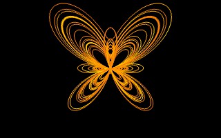
Figure 16.320. butterfly = exp(cos(t)) - 2*cos(4*t) - pow(sin(t/12),5)
Parametric curves program example : scale the butterfly at 1 and 0.5 : loop( 2 gscale(C/2))
Figure 16.322. Example for the Parametric Curves filter

Filter 'Parametric Curves' applied. Gauss family .
With this filter, you can create parametric curves and pictures. You can define points (x,y) in curves using the parametric functions x(t),y(t) or polar functions r(t) Using parametric functions, points are defined by their plane coordinates (x,y); using polar functions points are defined by their polar coordinates (r,t) where r is the radius (distance from origin) and t is the angle from the Ox axis. You may chose from either system.
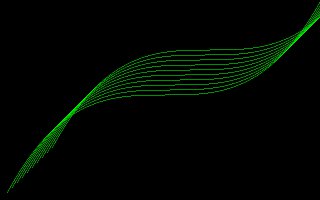
You can draw curves with various shapes, colors, gradients, rotate them, ..., make animated GIFs. The script comes with a library of various parametric or polar curves.
This filter allow to draw families of curves, each in its own layer. As usual with GIMP you can merge, delete, rotate, etc. curve layers for achieving best effects.
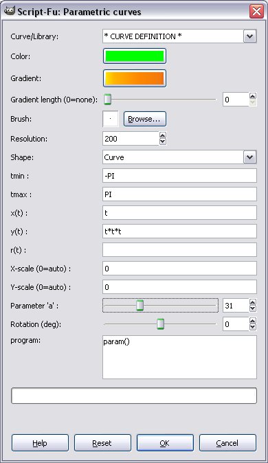
The Parametric Curves window let you chose curves from the library or program your own curves. He you will chose colors, shapes, .. and define curves functions.
Chose this item before entering the curve definition and parameters (see 13.23.3.2). Then press to draw the curve(s).
Chose a library curve then press to draw it. A pop-up message is displayed to show the library curve definition.
The 4 latest *user definitions* are saved in History-1 to 4. You can reload and replay one of them. History-1 is the last one drawn.
The dialog contains all options to set curves colors, calculation and select curve type (shape). Note that the script is able to draw at once a family of curves. See below, 'programming the curves' : loop(Cmax ...). Each curve is identified by C in [1..Cmax]. The variable C may be used in any function.
Colors and shapes
These options allow you to set color, gradient values and curves types (shapes)
The color value will be the foreground color for the curves drawing tools.
Select here a gradient for the brush tool.
If 0 no gradient is used. Else the gradient is repeteadly drawn with the specified length.
You can here for the type of brush to use for color or gradient, its Mode and Opacity.
With this drop-down menu You can chose what curve shape will be drawn, for instance: Curve, Radial, Dots, Steps, Path or Cartoon.
Standard curve: join the points with linear interpolation between two consecutive points.
Dotted line: draw only points, no line between them.
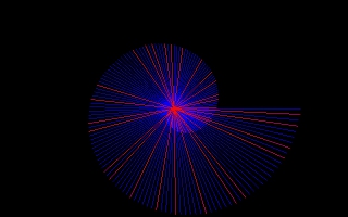
Radial: join the origin to the different points. Allows to 'fill' the curve. Nice effects is a gradient is used.
Step: To draw discrete (integer numbers) curves. see Fibonacci in the library.
Draws the curve in its own layer, then adds a path (SVG vector) to the image. You may then select, fill, edit, transform, export .. this path using the GIMP path tools.
Animated drawing from point 0 to last point. No gradient is used. You can set the speed = display refresh interval, with the cartoon(speed) function. See 'Logarithmic cartoon' in library. Shortened to 60 seconds if too long.
Curve Parameters
Input boxes to set curve functions definitions. Note that 'y(t)' means that y(t) is a function of t. It may depend upon other parameters (i=dot number, C=curve number, x, ..). It may even be constant. y=100 -> straight tight line.
Used to set the number of points (dots) that will be drawn. GIMP will perform linear interpolation between these dots. Each dot is indexed by i in [0..resolution[ . Any function may use the integer value i.
Most functions depend on t, which ranges from tmin (included) to tmax (included). Here you can set numerical values for tmin, tmax or use numerical expressions. For example : tmin = 0, tmin=-100, tmax = 2*PI, tmax = 1+log(PI), ...
Points (x,y) are defined by means of the two functions x(t) and y(t). These functions use standard math. notation (see below). Eg 1+sin(3*t), cos(sin(cos t))), etc. Caveat Do not write 'x = sin(t)+t' in the box, but'sin(t)+t'.
To define the curve by its polar definition r(t).r is the radius, i.e distance from origin for the angle t. Dilemn : if x(t),y(t) and r(t) definitions are given, r(t) is chosen.
Note : It is the exactly the same to write r(t) = f(t), where f is some function, or x(t) = cos(t)*f(t), y(t) = sin(t)*f(t). If f() is a complicated formula, you write it only once.
X-scale and Y-scale (pixels) give the maximum values for x and y along the axes. If X-scale = 0 (resp Y-scale = 0) the values are computed in order to fit to the window width (height). If polar coordinates are used, Y-scale is set to X-scale.
This slider sets the value of the variable named 'a' which may be used in curves definition. Usage : set 'a' and click OK (draw); set another value and redraw etc.
Defining the curves
These functions let you set define curves in ordinary mathematic notation. Eg : sin(t), cos(PI+3*t), ..
These functions may use the provided (read-only) variables x, y, t, R, ..
                Notations
                :=               is defined by
                -> n             function gives the result n
                [a..b]           closed interval. t in [a..b] means : a <= t <= b
                f(a,b)           function with two arguments a and b
                f(a[,b=666])     b argument is optional. Default value : 666

                == Operators ==
                * + - /          usual ops
                ^                exponentiation         3 ^ 3.34 -> 39.22699054
                %                modulo                 100 % 17 -> 15
                ()               used to group expressions when in doubt

                == Maths functions ==
                sin(x),cos(x),tan(x),log(x),acos(x),atan(x,y),...
                pow(x,y)         -> x^y
                exp(x)           -> E^x
                gauss(x [,s=1])  = 1/sqrt(2*PI*s) * exp(-x/(2*s))  gauss(0) -> 0.398..[Ref]
                normal(x)        = Int(gauss(x),-infinity,x)       normal(0) -> 0.5
                frand([x=1])     -> random value in ]-x..x[
                rand(n)          -> random integer value in [0..n[
                noise(x[,d=10])  -> random noise -> x +  frand(1)*x/d

                == Arithmetic functions ==
                floor(x)        floor(PI) -> 3
                ceiling(x)      ceiling(PI) -> 4
                int(x)          conversion to integer        int(PI) -> 3 ; int(-PI) -> -4
                uint(x)         conversion to integer > 0
                prime(x)        next prime > x        prime(4.5) -> 7
                gcd(m,n)        gcd(42,666) -> 6
                lcm(m,n)        lcm(42,666) -> 4662

                == If function ==
                if(test a b)    -> a if test is true, else b
                                Ex. C=3.  if(C > 4 sin(x) cos(x)) -> cos(x)

                == Test operators and functions ==
                &&, ||         and, or         if(((t>10) && (x<20)) ....)
                =, >, <                        if((t > 10) t (t-10)) -> 1 if t=11
                isprime(n)                      isprime(101) -> true
                even(n),odd(n)  is n even,odd ?


                == Variables ==
                i                step number = dot number in [0..resolution]
                tmin,tmax        bounds for time
                t                time in [tmin..tmax]

                x,y              curve (x,y )values at step i
                sx,sy            scaled values of x and y
                .x,..x           x at steps i-1, i-2        used for recurrences
                .y,..y           y at steps i-1, i-2        Ex. fibonacci : if((i < 2) 1 (.y + ..y))
                C                curve number in [1..Cmax]
                Rx,Ry            (pixels) x,y dimensions of screen from the origin
                R                = min(Rx,Ry) maximum visible radius
                a                variable set with the 'a' slider
                P(i)             other parameters (see 'programming the curves')
![[Tip]](images/tip.png)
|
Tip |
|---|---|
| The script will display information messages using GIMP pop-up messages. You can use the dialog to display/copy/.. the messages and curves definitions in the console window. |
Programming the curves
With the "program" textbox you can draw families of curves, script usual operations, dynamically override curves settings, and animate GIF's.Overriding of values applies to library or dialog curves. Yes, this is a script language inside the script-fu.
Eg. animate (38 FILL gscale(1-C/40) rotate(C*13)) - fig 16.325 -There are three program constructs :
The do(..) functions are the following, and are executed BEFORE the curve drawing. They may take into account the C curve number in [1...Cmax].
== Drawing ==
resolution(r)  Sets resolution to r >= 2
color(r,g,b)   Sets foreground (drawing) to (r,g,b)    color(0,255,noise(200))

sample(ith [,n=Cmax])
               Sets drawing color to i-th sample from the gradient.
               The gradient is sampled n times (default = Cmax)
               Ex :loop (10 sample(C)) -> colors 1 (beginning) to 10 (end) from the gradient

shape(s)       Defines the shape for the curve
               s = G_SHAPE_CURVE | G_SHAPE_DOTS | G_SHAPE_STEPS | G_SHAPE_RADIAL | G_SHAPE_CARTOON
               Ex : to draw a radial curve AND its enveloppe :
                      loop (2
                      when (C=1 shape(G_SHAPE_CURVE))
                      when (C=2 shape(G_SHAPE_RADIAL)))

cartoon(speed)     Sets shape to G_SHAPE_CARTOON and the speed for cartoon drawing
path(closed=0|1)   Sets shape to G_SHAPE_PATH. If closed=1 : close the path

== Geometry ==
gscale(s)              Global scale the image: x -> x*s, y->y*s
rotate(d)              Rotate d degrees around origin.         loop(4 rotate(90*C))
move(dx,dy)            Shifts the whole curve                  loop(10 move(10*C,20*C))
origin(orig)              Sets the origin for drawing. May be :
                       G_ORIGIN_0 (default, centered)
                       G-ORIGIN-CORNER (x >=0 and y >= 0)
                       G-ORIGIN-HALF-X (x >= 0)
                       G-ORIGIN-HALF-Y (y >= 0)

== Testing / Grouping actions ==
if (test true_do_this() false_do_that())
                      if ((C <  3) msg("In curve < 3 ",C) msg("In curve >= 3",C))

when (test do_this() do_that() ...)
                      when ((C > 10) rotate(C*78) move(10,42*C) msg("DONE",C))

== Miscellaneous ==
msg("title",v1,v2...) Message box to display v1,v2 ,.. values
                      Ex : loop(10 msg("Curve", C,secs()))
secs([0])             secs(0) -> init timer
                      secs() ->  elapsed seconds since init
verbose(level)        Displays curve information according to level = 0,1,2,3

== Curves parameters ==
                      A number of parameters  may be used in formulae for x(t,..), y(t,..) or r(t, ..).
                      This allows to draw families of curves.
P(i)                  -> returns value of parameter #i. i in [1...16]
P(i,v)                -> sets value v for parameter P(i). Return v.

Tips
                      Use ';' to comment out the program text
                      Ex.  ; loop (123 ...) -> no effect
Figure 16.326. r = exp(cos(t)) - 2*cos(4*t) - pow(sin(t/12),5)
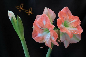
Add two layers to the flower picture, using the 'butterfly curve' from the library. Shrink, rotate and move these layers with the GIMP layers tools. It's done.
![[Note]](images/note.png)